TRECH

TRECH is a C++ simulation and learning toolkit that couples Geant4 particle transport with a stable, scriptable experiment layer and a provenance-first data trail. The core idea is simple: experiments can be authored in JavaScript, where scenarios can compute and compose configuration—covering unit conversions, dynamic assembly, and multi-entity layouts—before handing that configuration to the deterministic-by-default C++ runtime via JSON serialization.

In parallel, the runtime includes a lab command path that accepts live JSON commands like patch, simulate, snapshot, and quit. When simulate omits its count, TRECH measures the active scenario's wall time per round and learns the next batch size that fits lab.targetHz; explicit counts remain overrides. This enables interactive 3D-lab workflows without a fixed JS scenario file and makes their actual/planned precision machine-readable.

Prediction layers can relax determinism in a controlled way, with all changes logged in the provenance trail. The JS runtime utilizes a standard-compliant engine (QuickJS) which allows it to evolve without changing the configuration surface. To ensure accountability, hook registrations and deterministic callback dispatch points (init/run/event/step) are logged alongside run-level guardrails, patch/emit counters, hook-emit dropped counters, and hook-emit payload records.

Essential project points are:

• The simulation must relies less as possible on pre-determined physical and chemical formulas but has to obtain the behaviour at elementary particels level with GEANT4 and then changing simulation scale step by step determining statistical behaviours at larger scales. Physical and chemical laws can be used for comparison and validation purposes.
• TRECH has to costantly enforce GEANT4 simulation quality and statistical training and inference through ad hoc algorithms and using torch, learning when a prediction can be accurate and when is needed another statistical behaviour training on the run.
• That "scale step by step" idea is realized by the multi-scale inference cascade: scale-tagged learned models (models: [{name, path, scale}]) chained by the engine (ScaleCascade / ctx.cascade) from the Geant4 particle/nano base up the dimension ladder (atomic → nano → micro → meso → macro) to the observer scale — a general-purpose, context-driven predictor across every scenario family (fluids, chemistry, biology, CNT electronics, magnetic resonance…), not a set of narrow per-output models. See Multi-scale inference cascade.

Current stage: H2O baseline with optics/stratification, initial Geant4-DNA wiring, and nuclear cycle consistency analysis

The thesis in miniature: a biological cell clears lipophilic benzene while retaining polar D-glucose. PubChem XLogP and Geant4 membrane/cytosol plus event facts feed committed micro operators: ctx.evolve advances molecular transport and ctx.react decides conserved membrane crossings. No authored transport/crossing law runs on the default path; the retired formulas are validation-only teachers. The simulated count still matches the classical first-order curve at R²≈0.99, but that curve grades the learned microscopic result rather than driving it.

The thesis again, in an MRI: a 5 cm³ water cube in a static field. Geant4 builds the phantom + a copper receiver coil and — through the new material-composition surface (ctx.materials) — supplies the ¹H (proton) number density (6.686×10²² /cm³, exactly the literature value, never hard-coded); the deterministic hook layer runs the Bloch spin dynamics. We tell it only the proton gyromagnetic ratio γ (a particle constant) and the machine field B₀ — the resonance is not assumed. Left: a swept-RF spectroscopy pass locates a broad resonance; the precise Larmor line is DISCOVERED from the free-induction-decay carrier (the magnetization precesses at γB₀), recovering γ/2π = 42.5768 MHz/T vs CODATA 42.5775 (0.001%). Middle: the FID decays with a recoverable T2; its detected RF signal is the "output". Right: swap in NIST tissues and the Geant4-derived proton-density contrast falls straight out — adipose/muscle/brain near water, cortical bone the classic MRI-dark 0.58×. Geant4 does not simulate nuclear spin; the spin dynamics are hook-layer physics-for-comparison, and the textbook values grade the gap only. Render with tools/viz/demos/render_magnetic_resonance.py.*

Stage 2 makes the output photons REAL: for each NIST tissue the number of excitation primaries is set proportional to that tissue's Geant4-computed proton density (an "ignorant" material fact — Geant4 has no idea it's for NMR), Geant4 then produces every consequent photon (Compton scatter, fluorescence, secondary bremsstrahlung…), and a NaI detector shell scores the real deposited energy of all of it. The per-tissue detected signal (green) is thus a genuine Monte-Carlo tally, not a formula — and because the emission count came from Geant4's proton prediction, it reproduces MRI proton-density weighting: cortical bone lands at 0.60× water (the classic dark tissue), and the detected signal tracks proton density with r = 0.9995. The small bone gap (0.60 detected vs 0.58 proton ratio) is the honest radiographic photon-yield term. Multi-run driver scripts/run_magnetic_resonance_tissues.py; render with tools/viz/demos/render_magnetic_resonance_tissues.py.

Stage 3 turns the contrast into an actual image. Geant4 builds a real phantom — a row of NIST-tissue voxels along the readout axis, including an air gap (essentially no hydrogen, so no MR-visible ¹H protons — the signal comes from ¹H nuclei, not the protons bound in air's N/O/Ar nuclei) and cortical bone — and supplies each voxel's ¹H density. The hook layer applies a field gradient so the Larmor frequency becomes position-dependent (ω(x)=γ(B₀+G$_x$·x)), synthesizes the frequency-encoded readout, and DFT-reconstructs the 1D proton-density profile — a genuine MRI image line. Each voxel's position is recovered from its peak frequency to 0.001 mm (right panel, on the diagonal), the amplitudes track proton density (r = 1.0), and the image reads bright · bright · BLACK (air) · bright · dark (bone) · bright · bright. We feed only γ, B₀ and the gradient — the frequency→position map and the picture emerge. Render with tools/viz/demos/render_magnetic_resonance_imaging.py.

Stage 4 makes the picture a brain. A procedural, BrainWeb-inspired axial head phantom (skull, scalp/fat, CSF, cortical grey-matter ribbon, white-matter core, lateral ventricles) gives the anatomy; every pixel's brightness is the Geant4-computed mobile-¹H (proton) density of its tissue, and a 2D k-space acquisition + FFT reconstruct the image. The result is a genuine proton-density MRI: bright CSF and ventricles, grey matter brighter than white matter, bright fat rim, dark skull, black background — per-tissue intensity tracks the Geant4 proton density at r = 0.998. The anatomy is a digital phantom and the k-space/FFT is signal processing; the contrast is Geant4's. Render with scripts/run_magnetic_resonance_brain.py (needs numpy/matplotlib — use build/render-venv).

Why TRECH

• Reproducible: every run writes provenance (config JSON + hashes + seeds + versions).
• Determinism modes: strict simulation runs remain reproducible; predictive ML layers can be enabled with explicit provenance capture.
• Programmable: JS can compute and assemble configs (helpers, unit conversions, loops) while C++ remains in control.
• Extensible: initial Geant4-DNA physics wiring is available (guarded by TRECH_ENABLE_DNA_CHEM); chemistry and ML stubs remain.
• Agnostic config: long-term, keep the C++ config surface physics/chemistry agnostic while JS scenarios and lab sessions express combinations; define physics/chemistry classes, properties, and extensions in authoring layers.
• System abstraction: point-agnostic, ensemble-level metrics (densities) connect particle-scale runs to macro-scale predictions.
• Online learning: LibTorch/TorchScript is the chosen ML runtime for learning from simulation outputs (slower inference, but richer training loops).

Multi-scale inference cascade

The engine thesis made concrete: take a precise Geant4 particle/nano base and lift its behaviour, via statistical/ML inference, scale by scale up the dimension ladder (atomic → nano → micro → meso → macro) until it reaches the scale of the observer/experiment — so a macroscopic question ("what does this glass of water do while I stir it: the fluid motion, the waves?") can be inferred from the microscopic truth without hand-specifying every step.

Two tiers, both deterministic and disabled in strict mode (enabled in predictive):

• ctx.predict(name, features) — a single learned model (point-predictor); the scenario declares models: [{name, path}] and calls one model by hand.
• ctx.cascade(seed?, modelNames?) — chains declared models by their scale band (models: [{name, path, scale}]) in one pass: each stage's named outputs become the next-higher stage's inputs automatically, so lower-scale predictions feed higher-scale ones without the scenario wiring the chain. The optional name list selects one model family when the config also declares independent operators. Called with no argument it auto-seeds the bottom of the ladder from the real Geant4 base — the per-event tallies (edep_mev, track_length_mm, step_count, track_count, optical_photon_*) and, when materialProbe is on, the material.<name>.* probes (density, electron density, mean-I, X0, per-element number density) — so the scenario copies nothing from ctx.event/ctx.materials by hand; an explicit seed overrides/augments per key. Read the observer-scale prediction; it returns the flat, augmented context plus a __cascade trace (stages run, per-stage missing inputs, and the sorted seedKeys that seeded the pass).
• ctx.evolve(spec) — evolves arrays of named element state through learned operator stages. Operator models declare operator_role, element_kind, and required_context_keys; with no explicit model list the engine selects the single compatible role/kind group from the ambient Geant4/material context plus caller overrides. Ambiguous or absent matches return ran:false with a compatibility trace and do not mutate state. An explicit models list is still the override. Each N-element × K-stage pass reports N×K inferences.
• ctx.react(spec) — performs learned discrete transitions over integer state. The scenario declares species inventories, stoichiometric channels, and conserved linear quantities such as atoms, charge, or packet count; models emit bounded channel hazards. The engine owns deterministic seeded selection, rejects unavailable reactants without negative counts, and applies accepted deltas atomically. Reports distinguish model inferences, RNG draws, attempted transitions, accepted transitions, and availability rejections. Strict mode returns null without drawing or mutation. Its element_kind also accepts a per-element array, so one call can advance several materials at once: each kind selects its own operator from its own context, selection.groups[] reports what each material got, and a material with no compatible operator is left bit-identical instead of inheriting another material's law. ctx.react takes the same array (an unclaimed cell consumes no RNG draw), and ctx.interact selects per canonical pair kind — the unordered material combination of the two members (melt|sand), because a grain-grain, a grain-melt and a melt-melt contact are three different interactions.
• ctx.interact(spec) — the pair/neighbour operator: what one element does to another. The scenario declares positions, a neighbour cutoff and/or a persistent bond list, per-pair state, and which element fields receive contributions equal-and-opposite (antisymmetric — a force, a heat exchange) or shared (symmetric — a density/coordination sum). The engine owns the deterministic cell list, the canonical (a,b) enumeration, the exact equal-and-opposite application and the declared bounds; the learned stages own the interaction law. Reports P×K inferences over P pairs and K stages, with per-pair trust coverage. Mechanism shipped 2026-08-15; the MD/foam-bond/PBF migrations onto it are open roadmap rows, so no pair model is committed yet.

It is domain-agnostic — the same ScaleCascade serves every scenario family (fluids/H₂O, chemistry cycles, biology/membranes, CNT electronics, magnetic resonance, mechanics, nuclear); only the trained per-family stage models differ. Optics is merely the first family with a validated surrogate — not the point. Engine: include/trech/ml/ScaleCascade.{hpp,cpp}, ModelConfig.scale (conditionally serialized so existing config hashes hold), ctx.cascade + the ambient buildAmbientGeant4Seed in src/js/JsRuntime.cpp. Demo: cascade_multiscale_demo.js lifts a real Geant4 per-event energy deposit nano → meso to an observer-scale number — argument-free, its seed coming straight from the ambient Geant4 base.

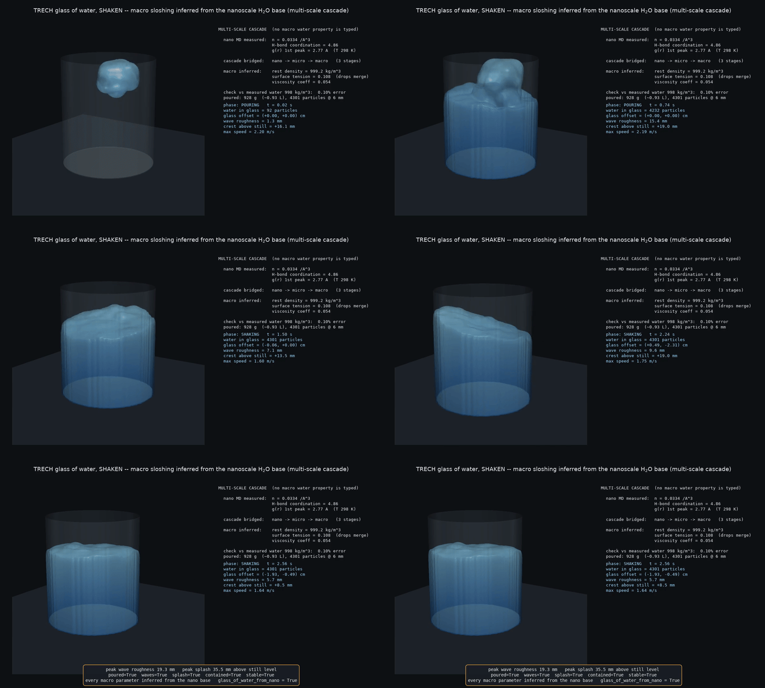
The section's own question, answered: glass_of_water_shaken.js pours ~1 litre of water into a glass, then shakes it — and never types a single macroscopic water property. A short rigid-SPC/E nano MD measures water's number density (0.0334 /ų) and hydrogen-bond coordination (≈4.86, g(r) peak 2.77 Å); ctx.cascade lifts those facts nano → micro → macro (3 bands in one pass) into the macroscopic fluid parameters — a rest density of 999.2 kg/m³ (a grounded coarse-graining of the nano number density, landing on measured water's 998 as a check, not an input — 0.10 % off), a surface tension (from the H-bond coordination) that merges drops on contact, and a viscosity. A Position-Based-Fluid solver (uniform spatial grid, ~4,300 particles at ~6 mm) then plays out three phases the video shows: water is poured in from a faucet and fills the wide tumbler (11 cm across, ~1 L), settles, and is shaken by a smooth-but-random motion. The 3D renderer draws the water as a 2 mm metaball isosurface so splashes break off and merge back into a cohesive body. Waves and splashes emerge, the water stays contained (mass conserved) and the run is stable — guarded by glass_of_water_shaken_waves. Render with tools/viz/demos/render_glass_of_water_shaken.py.

Honest scope: the Geant4 base is real; the inferred higher scales are learned/validated predictions (labelled as such, gap-to-truth measured). The demo stage models — both cascade_multiscale_demo's and the glass-of-water cascade's (data/glass_cascade/) — are illustrative maps that show the mechanism (the density coarse-graining is grounded; the cohesion/viscosity maps are labelled illustrative); the nano inputs are genuinely measured and no macro water property is typed. Training real, held-out-validated per-band chains across the scenario families is the standing objective in ROADMAP.md.

"Sputnik" milestone (north star)

108 periodic-box rigid-SPC/E water molecules (classical MD in the deterministic hook layer, SHAKE/RATTLE constraints, Geant4 as the per-tick clock) growing the O-O radial distribution function: the first peak lands at 2.74 Å vs the measured 2.80 Å hydrogen-bond distance, the inter-shell minimum (g≈0.78) and coordination (≈4.7) match the measured liquid, and the ~4.5 Å tetrahedral second shell is resolved. The same run measures the self-diffusion coefficient two independent ways — Einstein (MSD) and Green-Kubo (velocity autocorrelation) — which agree at D ≈ 2.6–2.8×10⁻⁹ m²/s, on the SPC/E literature value, with the VACF showing the dense-liquid cage-backscattering dip (h2o_self_diffusion.png, h2o_vacf_diffusion.png). A companion temperature sweep (h2o_diffusion_temperature.js) shows D(T) tracking the measured trend across 281–313 K (h2o_diffusion_temperature.png). Render with tools/viz/demos/render_bulk_water.py.

• Simulate H2O fluid behavior with Geant4 using as much subatomic detail as practical.
• Secondary reference ("Vostok" milestone): simulate carbon nanotube variants (structure, chirality, diameter) and electron behavior differences, including Fermi gap modeling, per docs/CNT/BackToTheCarbon.md. Electronic-structure step advanced: examples/experiments/cnt_band_structure.js reproduces the metallic/semiconducting classification ((n−m) mod 3 rule), the semiconducting primary band-gap ∝ 1/diameter law on STM-measured anchors, and the curvature-induced secondary gap for nominally metallic non-armchair tubes (E_curv ∝ |cos(3θ)|/d², armchairs remain zero-gap) via hook-layer tight-binding (cnt_band_structure.png). Logic-gate step landed: examples/experiments/cnt_logic_gates.js turns that band structure into working CNTFET devices and digital logic — the full static-CMOS gate family and half/full/2-bit-adder circuits whose simulated truth tables are confirmed against the canonical boolean/arithmetic functions, with the on/off ratio set by Fermi-Dirac statistics (~exp(E_g/2kT)), the recovered subthreshold swing on the ~60 mV/dec Fermi limit, and a metallic tube shown to short the logic. It now emits visual_topologies for each gate so cnt_circuit.gif renders NOT/BUFFER/AND/OR/NAND/NOR/XOR/XNOR from the scenario's CMOS networks instead of a fixed inverter-chain template (cnt_logic_gates.png; cnt_structure.gif / cnt_circuit.gif — see the scenario animation gallery).
• Learn to separate predictable events from exceptional ones so only outliers are re-simulated.
• Scale to large molecule counts with multi-scale acceleration (e.g., Lattice Boltzmann, variance reduction, reduced-order models).
• Prioritize photon transport accuracy (scattering, absorption, refraction, color response) within molecular volumes.
• "Apollo" milestone: totally generic physical simulator able to simulate and predict complex systems (chemistry on high volumes) and physical interactions

Architecture (short version)

1. Authoring input is either a JS experiment (run) or a live JSON command stream (lab).
2. C++ core parses config, applies deterministic patches/overrides, and tracks lab/session metadata.
3. Geant4 layer runs the canonical lifecycle and emits scoring + provenance.
4. System aggregation computes point-agnostic ensemble metrics for ML and multiscale stages.

See docs/structure.md for the detailed skeleton and docs/trech-roadmap.md for the full plan. Mermaid diagrams of the workflow, Geant4 wiring, prediction loop, and ML scale-up path live in CHARTS.md.

Quick start

git submodule update --init --recursive
cmake --preset dev
cmake --build --preset dev
./build/dev/trech run examples/experiments/hello_world.js
./build/dev/trech lab --config examples/lab/realtime_lab_bootstrap.json

Build artifacts live under build/ and are ignored by git.

CLI

trech run <experiment.js> [--macro <file>] [--ui] [--output <dir>] [--seed <n>] [--events <n>]
trech lab [--config <file>] [--commands <file>] [--output <dir>] [--seed <n>] [--events <n>]

Examples:

./build/dev/trech run examples/experiments/hello_world.js --output out
./build/dev/trech run examples/experiments/water_box.js --seed 42 --events 100
./build/dev/trech run examples/experiments/h2o_fluid.js
./build/dev/trech run examples/experiments/hello_world.js --macro examples/macros/minimal.mac
./build/dev/trech lab --config examples/lab/realtime_lab_bootstrap.json
./build/dev/trech lab --config examples/lab/realtime_lab_bootstrap.json --commands examples/lab/realtime_lab_commands.jsonl

lab mode command schema (JSON object per line, stdin or --commands file):

• {"action":"patch","patch":{...}} merge a config patch into the live session state.
• {"action":"simulate"} run Geant4 with the online timing planner's learned round count.
• {"action":"simulate","events":N,"seed":S} run Geant4 with an explicit one-command count override.
• {"action":"snapshot"} print canonical config plus lab.roundPlanner timing/precision state.
• {"action":"help"} print supported actions.
• {"action":"quit"} close the lab session.

The first batch initializes Geant4; compatible later batches reuse that kernel and call BeamOn directly. Event count, seed, and planner settings may change live. A patch to geometry, beam, physics, scoring, or output state is rejected after initialization with a restart-required error, because safe in-process reinitialization remains an explicit ROADMAP.md item. Always use achieved_hz, not the planned count alone, when describing real-time performance.

Config examples

• examples/experiments/hello_world.js: minimal baseline.
• examples/experiments/water_box.js: container volume holding explicit water material (non-chemical boundary).
• examples/experiments/config_optics.js: medium box with optics enabled (includes optics.spectrum sample) and explicit water material.
• examples/experiments/h2o_fluid.js: H2O fluid stub with container + brine mixture + nested solute seed.
• examples/experiments/h2o_single_molecule.js: single-molecule proxy stub with container + nested sphere proxy.
• examples/experiments/h2o_optics_beam.js: optical photon beam through water (spectrum-enabled, explicit water material).
• examples/experiments/config_stratify.js: event stratification thresholds/labels.
• examples/experiments/config_stratify_ml.js: stratification with TorchScript model path stub.
• examples/experiments/surrogate_generic_demo.js: generic learned inference — declares a models: [{name, path, scale}] entry and calls it via ctx.predict(name, features) (a single point-predictor; here the committed optics ridge predicts water's refractive index).
• examples/experiments/cascade_multiscale_demo.js: multi-scale inference cascade — declares two scale-tagged models and lets ctx.cascade(seed) chain them from a real Geant4 per-event energy deposit (nano) up to an observer-scale response (meso) in one pass, with no hand-wiring. Illustrative stage models under data/cascade_demo/ demonstrate the mechanism (see Multi-scale inference cascade).
• examples/experiments/glass_of_water_shaken.js: the cascade's canonical worked example — a glass of water poured and shaken. A short rigid-SPC/E nano MD measures water's number density + hydrogen-bond coordination; ctx.cascade lifts them nano→micro→macro into the macroscopic fluid parameters (rest density 999 kg/m³ — a grounded coarse-graining that lands 0.1% off measured water without typing it; a cohesion that merges drops; a viscosity); a Position-Based-Fluid solver (uniform spatial grid, ~4,300 particles at ~6 mm) then pours ~1 L of water into a wide glass (11 cm across), lets it settle, and shakes it, producing waves + splashes that stay contained. No macroscopic water property is hand-typed. 3-band cascade + illustrative stage models under data/glass_cascade/; rendered as a 2 mm metaball isosurface by tools/viz/demos/render_glass_of_water_shaken.py; guarded by glass_of_water_shaken_waves.
• examples/experiments/beaker_water_n_pentane.js: water + n-pentane poured into an open beaker at 30 °C and observed for 60 minutes. Geant4 NIST materials supply composition/density and the cross sections behind TRECH's colour/optics; PubChem supplies CID + SMILES structure only. A two-stage ctx.cascade consumes that ambient base plus beaker/air context and infers colour, phase separation/layer order, temperature-aware held-out volatility and evaporation. At 303.15 K, 100 mL water + 50 mL n-pentane are inferred colourless with pentane above water; predicted vapour pressure is 87.17 kPa vs validation-only NIST 81.98 kPa (6.3%), and 13.99% / 4.38 g evaporates in 60 min. Sixty-one material_frames now show an empty beaker → water pour → pentane pour → transient intermingling/phase separation → a moving, fading vapour plume; the physical 60-minute interval is retained beside an explicit 545× playback clock. Optional tints/vapour emphasis are tagged representation-only. Guarded by beaker_water_n_pentane_inference (11 checks). The macro response surface and hook-layer kinematics remain illustrative with σ=0.08; a wider liquid-pair/airflow panel is tracked in ROADMAP.md.
• examples/experiments/lava_lamp.js: a duration-independent, stateful 3D lava-lamp thermofluid scenario. Geant4 probes water and a configured paraffin/density-modifier reference blend; the two-stage ctx.cascade infers melting, thermal expansion, heat transfer/diffusion, viscosity/drag, cohesion, interfacial velocity coupling, carrier circulation/advection, vorticity, and lateral-plume strength. A bounded-step solver advances persistent parcel IDs through temperature, liquid fraction, density, buoyancy, a cylindrical 3D convection basis, velocity coupling, boundaries, and neighbour topology—without a target cycle, authored trajectory, preferred axis, phase schedule, birth, or regeneration. Initial thermal fluctuations deterministically choose the convection orientation and handedness. The README run's centroid spans 38.73 mm × 36.52 mm laterally, traverses 123.41 mm, and visits 10/12 azimuth sectors. Its earlier fine parcel interface is preserved independently at 19 coalescences, 18 fissions, and 43/101 merged states; a wider observer-scale Gaussian interface adds distance-faded in-gap splats only for parcel pairs already inside its connection radius, producing continuous neck growth/rupture with 8 merges, 10 splits, and 90/101 merged states. The Studio GIF and classic 3D GIF show the complete 600 s response in ten seconds; both viewers share this contract and never move centres or change component topology. Precision remains split across fixed-volume parcel count, max_physics_step_s integration, simulation_ticks sampling, and representation-only render_surface_grid_mm. Emitted centres and clocks are unchanged; 100 post-tick states map directly to 100 GIF frames with no interpolation or optical flow. Guarded by lava_lamp_inferred_thermofluid (23 checks), including retained parcel lineage, fluid-interface merge/split lineage, volumetric non-axis-locked transport, temporal coherence, duration/condition, and precision refinement. Geant4 does not itself solve phase change or CFD; the compact response and parcel discretisation remain illustrative, with wider held-out training tracked in ROADMAP.md.
• examples/experiments/config_chemistry_stub.js: chemistry/DNA wiring (DNA physics when enabled; chemistry stage still stubbed by default).
• examples/experiments/config_multiscale_stub.js: multi-scale stub wiring config.
• examples/experiments/config_nitrogen_carbon_cycle.js: nitrogen gas <-> carbon-14 cycle scenario (N-14 + n -> C-14 + p, C-14 -> N-14 + e- + anti_nu_e) with Geant-backed consistency/Q-value reporting.
• examples/experiments/analytic_beer_lambert.js: complex test scenario with a classical-formula cross-check — a narrow 100 keV gamma beam through a 50 mm water slab, where the engine compares the textbook Beer-Lambert prediction T = exp(-mu*x) (with mu summed from Geant4's own atomic cross sections via G4EmCalculator) against the run's measured Monte-Carlo uncollided-primary fraction. Both numbers + the gap land in trech_scores.jsonl under analytic_checks (classical 0.4265 vs Geant4 0.4217, ~1.1% — Poisson-limited).
• examples/experiments/analytic_csda_range.js: charged-particle CSDA-range cross-check — a 20 MeV proton fully stops in water; the engine derives the CSDA range from Geant4's own stopping power (G4EmCalculator::GetCSDARange) and compares it to the measured mean primary track length (a new per-primary path-length tally). Derived 4.28 mm vs measured 4.27 mm (~0.4%); emitted under analytic_checks (type: "csda_range"), guarded by analytic_csda_range_cross_check.
• examples/experiments/analytic_photo_fraction.js: photon process-branching cross-check — a 30 keV gamma beam (near water's photoelectric/Compton crossover) where the engine predicts the photoelectric share of the total interaction cross section sigma_phot/sigma_total from the same G4EmCalculator cross sections and compares it to the measured fraction of primaries whose first discrete interaction is photoelectric (classified through QBBC's G4GammaGeneralProcess wrapper by EM subtype). Derived 0.391 vs measured 0.393 (~0.6%); emitted under analytic_checks (type: "photo_fraction"), guarded by analytic_photo_fraction_cross_check. Unlike the attenuation/range checks, this tests the process choice and is slab-thickness independent.
• examples/experiments/config_cnt_stub.js: CNT stub modeled in a fluid container with explicit materials and nested volumes.
• examples/experiments/config_cnt_world_stub.js: CNT stub volume placed in a void container in the world (no medium box).
• examples/experiments/config_cnt_optics_stub.js: CNT geometry + optics mixed testing stub (medium box + optics enabled).
• examples/experiments/cnt_band_structure.js: CNT electronic-structure comparison panel; emits metallicity, primary semiconducting gaps, curvature secondary gaps for quasi-metallic tubes, and validation flags to trech_hook_emits.jsonl.
• examples/experiments/cnt_logic_gates.js: CNT logic gates + circuits — builds CNTFETs from the tight-binding band gap, the full static-CMOS gate family (NOT/BUFFER/AND/OR/NAND/NOR/XOR/XNOR as resistive-divider pull-up/pull-down FET networks), and three circuits (half adder, full adder, 2-bit ripple-carry adder), then confirms the truth table the electrons produce at every output. The transistor on/off ratio is Fermi-Dirac-set (~exp(E_g/2kT)), the subthreshold swing recovered from the simulated I_d(V_gs) lands on the ~60 mV/dec room-temperature Fermi limit, and a metallic tube dropped into the same topology collapses the outputs to ~Vdd/2 and breaks the logic (the metallic-short manufacturing problem of docs/CNT/BackToTheCarbon.md). Geant4 transports the e- beam through the representative (16,0) channel each event. Emits cnt_device + cnt_gates_summary with visual_topologies and visual_source; rendered by tools/viz/demos/render_cnt_logic_gates.py → cnt_logic_gates.png and tools/viz/demos/render_cnt_circuit.py → cnt_circuit.gif; guarded by the cnt_logic_gates case.
• examples/experiments/config_flow_language.js: flow-style scenario using TRECH_FLOW chaining (set, defaults, merge, push, derive, ensureArray, normalizeDetectorAliases, finalize, require) and function-based TRECH_CONFIG.
• examples/experiments/config_hook_dispatch.js: hook runtime smoke example (ctx, deterministic emit, onInit override patch, and hook guardrails: hooks.maxStepCallbacks, hooks.maxEmitsPerCallback, hooks.maxEmitPayloadBytes).
• examples/experiments/testscenario_efflux.js: headline biological comparison — a cell clears lipophilic benzene through a lipid bilayer while retaining polar D-glucose. The default path no longer contains an authored transport or membrane-crossing law: ctx.evolve advances each molecule through the committed micro transport model and ctx.react owns the learned crossing hazard, seeded draw and packet conservation. PubChem XLogP and Geant4 membrane/cytosol interaction plus event facts are model inputs. The retired OU/advection/drift and Overton-scaled crossing formulas run only with physics_source=reference. The operator run retains all 30 glucose packets, clears 76/80 benzene packets and fits first-order clearance at R²=0.984; efflux_operators_match_reference passes all four observer gaps and 22/22 trust checks with zero out-of-domain inferences.
• examples/experiments/glass_from_sand.js: a material that does not exist when the run starts. Geant4 builds and probes silica sand, soda ash, limestone and the declared soda-lime product; a nano→macro cascade turns those facts into this batch's calcination/melt/fusion onsets and its conduction coefficient (no onset is typed into the scenario); then per-material ctx.evolve, per-material ctx.react and per-pair-material ctx.interact advance each cell with the operator its CURRENT material class selects, as cells migrate batch_solid → melt → glass. The chemistry is real stoichiometry — Na2CO3 → Na2O + CO2, CaCO3 → CaO + CO2, 6 SiO2 + Na2O + CaO → Na2O·CaO·6SiO2 — with Si/Na/Ca/C/O conservation validated by the engine before any draw. The nominal run creates 108 glass units from zero, closes every element balance at exactly 0, never reacts below an inferred onset, and forms its first glass at the bottom of the charge because heat only enters at the floor. Its five per-material operators are distilled trained artefacts (physics_source=operator, the default): harvested from the states five independent furnace operating points actually visited, held out by whole run on two never-fitted ones, and carrying a measured meso hull, occupancy, band and held-out metrics. The hand-authored family they came from is reachable as physics_source=reference and remains the teacher — so the near-unit held-out R² is migration fidelity, not physical accuracy (measured:false), and the onsets/conductances stay illustrative. Guarded by glass_from_sand_material_creation (21/21) and the paired glass_operator_matches_reference (8/8 gaps, 22/22 trust).
• examples/experiments/testscenario_h2o_electrolysis_combustion.js: H2O reaction-cycle test — the default ctx.react path evaluates a committed meso hazard model over 90 two-water reaction cells, while the engine owns seeded choices, availability, atomic mutation and exact declared H/O conservation. PubChem supplies formulas/CIDs; raw Geant4 event and G4EmCalculator interaction facts condition the learned hazards. It produces 180 H2 + 90 O2 across two cathodes and recovers all 180 waters with zero out-of-domain inference. The former electrolysisProbability/combustionProbability laws survive only as reaction_source=reference audit teachers. Guarded by both h2o_electrolysis_combustion_cycle and the 4/4-gap, 22/22-trust h2o_cycle_operator_matches_reference pair.
• examples/experiments/briggs_rauscher_oscillator.js: the Briggs–Rauscher oscillating reaction in an open beaker — the classic chemical clock that visibly cycles colourless → amber → deep blue-black → colourless for minutes, then settles. TRECH is told only what is in the beaker: the reagent recipe (KIO₃ / H₂O₂ / malonic acid / H₂SO₄ / MnSO₄ + starch, as molarities) and the Geant4-constructed solution materials. Geant4 reports the dissolved iodine (1.5e20 /cm³) and manganese (6.9e19 /cm³) and the colourless solution's derived colour; a two-stage ctx.cascade (nano reagent descriptors → macro observer-band response) infers the coefficients of a reduced Field–Körös–Noyes / Oregonator relaxation oscillator (f, ε, q, iodide regeneration/consumption, iodine production/removal, triiodide–starch coupling, reservoir depletion, seconds-per-τ). The cascade emits no period, cycle count, colour, or phase schedule: a deterministic hook-layer integrator advances the oscillator plus the emergent [I₂]/[I⁻] species, and the oscillation itself emerges — 8 completed colourless→amber(free I₂)→deep-blue(triiodide·starch) cycles with amber always preceding blue, a ~10.5 s period, then a clean settle when the oxidant/substrate reservoir depletes (all graded against known Briggs–Rauscher behaviour only at run end). Emits br_frame (beaker colour, [I₂]/[I⁻], cycle index) + briggs_rauscher_summary; rendered by tools/viz/demos/render_briggs_rauscher.py → briggs_rauscher.gif; guarded by briggs_rauscher_oscillation (10 checks). Honest scope: Geant4 does not solve aqueous radical/non-radical iodine chemistry — the reduced oscillator is a labelled "physics for comparison" hook-layer model whose coefficients are inferred from the Geant4 base; the compact macro response surface is illustrative (σ=0.12 emitted), and the amber/blue-black swatches are labelled representation while the colour timing/sequence is the emergent, graded result. A wider trained oscillating-chemistry panel is tracked in ROADMAP.md.
• examples/experiments/polyurethane_foam.js: the polyurethane foam experiment ("the solid sponge") — two viscous liquids are poured into a cup (Solution A: polyol + a little water; Solution B: a diisocyanate) and within seconds the mixture creams, expands toward ~30x its volume, and cures into a rigid porous sponge that leans under its own weight, cracks, and drops pieces onto the table. TRECH is told only what is in the cup: the two-part recipe and the Geant4-constructed solution materials. Geant4 reports the isocyanate nitrogen in Solution B, the A/B density contrast, and the mixed liquid's derived colour; a two-stage ctx.cascade infers the coefficients of both the dual-reaction chemistry — gel (R−N=C=O + R'−OH → urethane) and blow (R−N=C=O + H₂O → amine + CO₂↑) — and the mechanics of the foam it builds (bond stiffness, failure strain, stress relaxation, material drag, contact, and the cell-scale imperfection dispersion). Every parcel then runs its own chemistry, with heat diffusing along the bond network and leaking from the free surface, so a hot core and a cooler skin appear on their own. The material is a growing viscoelastic bonded-parcel network under standard gravity (trech_foam_solver.js): rest lengths grow with each parcel's gas generation, creep away stress while fluid, lock as it cures, and break past the failure strain — so the cream, the rise, the exotherm, the cream→gel→solid ordering, the lean, the cracks, which pieces detach and where they land are all consequences, never scheduled. A gravity_scale=0 control run must produce no fallen debris and less lean and cracking, proving gravity caused the sag rather than a script. PubChem contributes structure identity only (CID+SMILES+formula, element-cross-checked). Rendered by classic trech-viz → polyurethane_foam.gif; guarded by polyurethane_foam_expansion. Honest scope: Geant4 solves neither urethane kinetics nor continuum mechanics — both are labelled "physics for comparison" hook-layer models whose coefficients come from the Geant4-seeded cascade, gravity is used as a physical constant, the macro response surface is illustrative, and fracture siting is discretisation-sensitive (the aggregate response is what is guarded). Remaining work — training those coefficients instead of hand-authoring them, and a mesh-objective fracture criterion — is tracked in ROADMAP.md.
• Engine-side polyurethane reaction operator: the promoted default (chemistry_source=operator) moves the eight-field per-parcel chemical update out of scenario JavaScript and through StateEvolution/ctx.evolve. The committed meso MLP (data/polyurethane_cascade/meso_reaction_operator.json, 2,216 parameters) was trained on 115,437 rows spanning 285–310 K and 0.02–0.08 s steps and validated on 38,565 independent-run rows (worst-output R²=0.9929). It carries teacher=polyurethane_foam.js and measured:false: this is the reduced model learned, not new measured foam physics. polyurethane_operator_matches_reference passes all eight paired observer gaps (0.56% expansion; ≤1.07 s milestone drift; 1.19 K core-skin drift), with all 2,812,320 parcel-step inferences in-domain; the chemical→mechanical coupling and solver laws remain authored and tracked in ROADMAP.md. Its model is selected contextually from operator_role=reaction_state, element_kind=foam_parcel, and its 16 required shared facts; the same declarative paired-run validator now gates future scenario migrations.
• examples/experiments/elephants_toothpaste.js: elephant's toothpaste ("the soapy lather") in a graduated cylinder — concentrated H₂O₂ + dish soap meets a KI solution and the iodide-catalysed decomposition 2 H₂O₂ →(I⁻) 2 H₂O + O₂↑ erupts as a massive steaming lather column that never solidifies. TRECH is told only what is in the cylinder: the recipe (30% peroxide, 2% soap, 2 M KI, pour fractions) and the Geant4-constructed solution materials. Geant4 reports the dissolved iodine (1.30e21 /cm³) and potassium (1.29e21 /cm³), the oxygen-rich peroxide density (1.11 g/cm³), and the clear mixture's derived colour; a two-stage ctx.cascade infers the coefficients of a reduced catalytic-decomposition model (catalysed + uncatalysed rate constants, Arrhenius activation, exotherm, O₂ foam capacity, surfactant trapping, lather drainage, iodine-intermediate shunt). The cascade emits no completion time, eruption height, temperature, or colour: the hook-layer integrator makes it all emerge — an 80,000× catalytic acceleration, 90% completion in 9.7 s, the foam over the rim in under a second, a 18.4× lather column 433 mm above the rim, a steaming sub-boiling 368.9 K peak (an explicit, labelled evaporative clamp near the carrier boiling band accounts for only 8.2 K of that — the unclamped exotherm would reach 375.7 K, and both numbers are emitted so the clamp's share is measured, not hidden), a transient amber iodine tinge that fades as the peroxide depletes, and a soft lather that keeps moving and drains to 74% of peak without ever rigidifying — the emergent consistency contrast to the polyurethane sponge (graded against known demonstration behaviour only at run end). PubChem contributes structure identity only (H₂O₂/KI/water CID+SMILES+formula, element-set cross-checked). Emits 136 material_frames + elephants_toothpaste_summary; rendered by classic trech-viz → elephants_toothpaste.gif; guarded by elephants_toothpaste_eruption (16 checks). Honest scope: Geant4 does not solve aqueous redox kinetics or foam drainage — the reduced model is a labelled "physics for comparison" hook-layer model whose coefficients are inferred from the Geant4 base; the compact macro response surface is illustrative (σ=0.15 emitted), and the white/amber swatches are labelled representation while their timing is the emergent, graded result. A wider trained catalytic-kinetics panel is tracked in ROADMAP.md.
• tools/pubchem (python -m trech_pubchem fetch <names>): PubChem property + 2D-structure cache helper. Use --cache-dir or TRECH_PUBCHEM_CACHE_DIR for build-local real-time fetches (the validation suite uses build/dev/pubchem_cache); new fetched records are ignored by git by default.
• examples/experiments/testscenario_magnetic_resonance.js: magnetic resonance (Stage 1) — NMR/MRI of a 5 cm³ water cube. Geant4 builds the phantom + a copper receiver-coil volume and, through the new material-composition surface (materialProbe/ctx.materials), supplies the ¹H (proton) number density that sets the equilibrium magnetization; a G4EmCalculator beer_lambert anchor + per-event transport are the clock. The deterministic hook layer runs the Bloch spin dynamics: a swept-RF spectroscopy pass and a free-induction-decay pass whose lab-frame carrier is measured to discover the Larmor line — feeding only the proton gyromagnetic ratio γ (a particle constant) and the machine field B0, so γ/2π = 42.5768 MHz/T (vs CODATA 42.5775, 0.001%), the Geant4 water proton density 6.686e22/cm³ (= literature, 0.006%), and T2* all emerge and are graded against the textbook values. mr_summary.tissue_preview already shows the Geant4-derived proton-density contrast (cortical bone 0.58× water) for the upcoming tissue stage. Emits mr_spectrum/mr_fid/mr_summary; guarded by magnetic_resonance_water. Honest scope: Geant4 does not simulate nuclear spin — the spin dynamics are hook-layer physics-for-comparison.
• examples/experiments/testscenario_magnetic_resonance_tissues.js + scripts/run_magnetic_resonance_tissues.py: magnetic resonance (Stage 2) — virtual-tissue contrast with REAL Geant4 photon emission (multi-run, no C++). The driver reads each NIST tissue's Geant4-computed ¹H number density from material_probes (an ignorant material fact), runs the scenario per tissue with the excitation-primary count set proportional to that proton density, and Geant4 then produces every consequent photon which a NaI detector shell scores as real deposited energy (receiver_coil volume_edep_mev). The per-tissue detected signal is a genuine Monte-Carlo tally that reproduces MRI proton-density contrast (cortical bone 0.60× water, corr 0.9995), byte-reproducible. Aggregate emitted as mr_tissue_contrast; guarded by magnetic_resonance_tissue_contrast. Honest scope: the excitation-per-proton is a labelled proxy (Geant4 can't make spins radiate RF); what is REAL is the Geant4-set emission count and the Geant4-transport detection tally.
• examples/experiments/testscenario_osmotic.js: validation scenario for a biological cell osmotically dehydrating in a hypertonic bath (docs/testscenario_osmotic-todo.md); a coarse-grained 2D MD bath of H2O + glucose + wrong-polarized ions around a selectively permeable, turgor-driven spring membrane runs inside the hook layer (one Geant4 event = one MD tick). A Langevin thermostat keeps the 310 K kinetic proxy bounded while the cell expels water through its pores, crenates (the membrane contracts and buckles as water leaves — an emitted physical state), and expels wrong-polarized molecules (glucose by size, small ions by polarity). final_summary validates 9 behaviours — dimensional + polarity exclusion, early pore crossings, macroscopic water flux, osmotic shift, bounded energy, late pressure bias, membrane crenation and stability. osmotic_particles emits (positions, polarity, membrane node radii, expelled strikes) feed tools/viz/demos/render_osmotic.py for an evident-cell replay video, with no fixed osmotic law driving the animation.
• examples/experiments/testscenario_pascal.js: validation scenario for Pascal's principle and material deformation (docs/testscenario_pascal-todo.md); three vessel models (ideal-rigid, Hookean/plastic, finer micro/macro structural mesh) are advanced through thermalize → baseline → compress → hold → release phases with per-bucket deterministic initialization, emitting live pressure windows, wall profiles, elastic/plastic displacement, and pascal_summary flags (pascal_principle_holds, plastic_damping_observed, macro_mesh_consistent).
• examples/experiments/trech_helpers.js: JS helper module (units, constants, material presets, geometry helpers).
• examples/experiments/config_multi_beam_units.js: unit conversion + multi-beam composition example (uses beams array normalization).
• examples/experiments/include_error_demo.js: TRECH_INCLUDE stack demo (intentional failure via include_error_helper.js).
• examples/lab/realtime_lab_bootstrap.json: JSON bootstrap config for trech lab (no JS authoring required).
• examples/lab/realtime_lab_commands.jsonl: sample real-time lab command stream (patch/simulate/snapshot).

Helper modules are single-file today; load them with TRECH_INCLUDE("trech_helpers.js") to keep line numbers stable.

Optics can be constant or spectral. Use optics.spectrum with energyEv or wavelengthNm entries to override refractive index/absorption/scatter per wavelength while keeping the config JSON canonical. H2O stubs author system blocks in JS to label ensembles and keep aggregation point-agnostic.

CNT runs are still a parallel track for schema/physics coherence, but they now use the generic geometry.volumes surface. Volumes declare shapes (box/tube/sphere), materials, placements, and optional scoreEdep flags. The CNT stubs steer the beam across a tube shell volume to exercise volume_edep_mev while keeping comparisons focused on electron transport; photon counts are a secondary comparison in mixed tests.

Essential test scenarios

This is the canonical set of physics/chemistry scenarios the validation suite exercises, grouped by how much each one learns from Geant4 vs. relies on a pre-written law. The project thesis (see the top of this file) is to obtain behaviour from Geant4 particle transport and use classical formulas only for comparison/validation — so each scenario below is labelled with Geant4's role. Re-run them all and regenerate docs/validation_report.md with scripts/run_validation_suite.sh; each row's validation case is the pass/fail guard. Honest scope is stated per tier — Geant4 transports particles but cannot itself form bound molecules, compute band structure, or evolve a chemical network, so those tiers use a hook-layer model with Geant4 as an anchor/clock, never a fitted rule standing in for the physics.

Every scenario below has an evident animation under tools/viz/demos/ (e.g. cnt_structure.gif/cnt_circuit.gif — nanotubes with electrons flowing and a panning CNTFET circuit; csda_bragg.gif — a proton stopping at its Bragg peak; beer_lambert.gif, h2o_molecule.gif, electrolysis.gif, …). See tools/viz/demos/README.md; regenerate with render_physics_anims.py + the per-scenario renderers.

Tier 1 — behaviour derived from Geant4 (no pre-written physical law drives the result; the classical formula is only the cross-check):

Scenario	Validates	Geant4 role	Validation case
viz_refraction_demo.js	refractive index n(λ) of air/water/glass, ordering, n ≥ 1, KK window	G4EmCalculator photo/Compton/Rayleigh cross sections → Beer-Lambert extinction → Kramers-Kronig dispersion → n. No n is ever hardcoded.	optics_n_water/glass/air, optics_index_ordering, optics_index_above_one, optics_kk_integration_window
analytic_beer_lambert.js	photon attenuation T = exp(-μx)	μ summed from Geant4's own atomic cross sections; classical T vs the run's measured Monte-Carlo uncollided-primary fraction (≈1% gap)	analytic_beer_lambert_cross_check
analytic_csda_range.js	charged-particle range R_CSDA = ∫dE/(dE/dx) (20 MeV proton in water)	CSDA range from Geant4's own stopping power (GetCSDARange) vs the run's measured mean primary track length (a per-primary tally); ≈0.4% gap	analytic_csda_range_cross_check
analytic_photo_fraction.js	photon process branching f = σ_phot/σ_total (30 keV gamma in water)	photoelectric fraction from Geant4's own per-process cross sections vs the run's measured fraction of primaries whose first interaction is photoelectric (G4GammaGeneralProcess sub-process by EM subtype); ≈0.6% gap	analytic_photo_fraction_cross_check
config_nitrogen_carbon_cycle.js	nuclear cycle N-14 + n → C-14 + p, C-14 → N-14 + e⁻ + ν̄	Geant4 isotope masses → Q-values + charge/baryon conservation	nuclear_cycle_conservation, nuclear_cycle_q_value_closure

Tier 2 — Geant4-anchored mesoscale (a hook-layer model whose rate/selectivity is scaled by live Geant4 data; validated against a closed-form law):

Scenario	Validates	Geant4 role	Validation case
testscenario_efflux.js	passive membrane efflux → first-order clearance N(t)=N₀e^{-kt} (validation only)	micro ctx.evolve transport + ctx.react crossing models consume PubChem/Geant4 context; retired JS laws are reference-only	efflux_first_order_kinetics, efflux_operators_match_reference
glass_from_sand.js	sand + soda ash + limestone under furnace heat → soda-lime glass (a material created mid-run)	Geant4 material probes → cascade onsets; distilled trained per-material ctx.evolve/ctx.react operators (reference teacher retained) and per-pair-material ctx.interact; engine-enforced Si/Na/Ca/C/O conservation	glass_from_sand_material_creation, glass_operator_matches_reference
testscenario_h2o_electrolysis_combustion.js	electrolysis + inverse combustion: 2 H₂O → 2 H₂ + O₂ → 2 H₂O	meso ctx.react model predicts hazards; engine enforces atom conservation and seeded transitions; JS formulas are reference-only	h2o_electrolysis_combustion_cycle, h2o_cycle_operator_matches_reference
briggs_rauscher_oscillator.js	Briggs–Rauscher oscillator: colourless→amber→deep-blue cycling emerges from the beaker recipe alone — 8 cycles, amber-before-blue, ~10.5 s period, then settles on reagent depletion	Geant4-built solution materials report the dissolved I + Mn and the colourless colour; a two-stage cascade infers the Oregonator coefficients — the oscillation/period/colours are emergent, not typed	briggs_rauscher_oscillation
polyurethane_foam.js	polyurethane foam ("the solid sponge"): cream→rise→gel→solid from the two-part recipe alone, plus the gravity consequences — the bun leans under its own weight, cracks, sheds pieces, and the pieces land on the table; a zero-g control prevents any piece reaching the table and sharply reduces detachment, lean and cracking	Geant4-built solution materials report the isocyanate N + A/B density contrast + liquid colour; a two-stage cascade infers coefficients, the promoted-default trained ctx.evolve operator replaces the per-parcel JS reaction law, and a bonded-parcel network under standard gravity is integrated	polyurethane_foam_expansion, polyurethane_operator_matches_reference
elephants_toothpaste.js	elephant's toothpaste ("the soapy lather"): an 8e4× iodide-catalysed runaway, 90% done in 9.7 s, an 18.4× steaming lather column 433 mm over the rim (369 K), transient amber iodine tinge, then slow drainage — never solidifies	Geant4-built solution materials report the dissolved I + K, the O-rich peroxide density, and the clear colour; a two-stage cascade infers the catalytic-decomposition coefficients — acceleration/eruption/steam/drainage are emergent, not typed	elephants_toothpaste_eruption
beaker_water_n_pentane.js	sequential pour/intermix/separate, colourless immiscible pentane upper layer, and temperature-aware 30 °C / 60-minute evaporation (13.99% / 4.38 g, σ=0.08) with a moving vapour plume	Geant4 NIST material/optics facts auto-seed a two-stage cascade; PubChem contributes CID+SMILES only; physical/chemical references grade the result only	beaker_water_n_pentane_inference
lava_lamp.js	Persistent wax parcels integrate heat, phase, density, buoyancy, drag, cohesion, and neighbour topology; duration is only the horizon	Geant4 water/reference-blend material+optics facts seed a two-stage cascade whose inferred coefficients are consumed at every bounded physics step	lava_lamp_inferred_thermofluid
testscenario_magnetic_resonance.js	NMR/MRI of a 5 cm³ water cube: hook-layer Bloch dynamics discover the Larmor line (γ/2π = 42.577 MHz/T, 0.001% gap) from the FID carrier; signal scaled by proton density	Geant4 builds the phantom + receiver coil and, via the new material-probe surface (ctx.materials), supplies the ¹H (proton) number density (6.686e22/cm³ = literature); G4EmCalculator beer_lambert anchor + per-event clock	magnetic_resonance_water
testscenario_magnetic_resonance_tissues.js + driver	MRI tissue contrast, REAL photons: per NIST tissue the excitation count ∝ Geant4's proton density, Geant4 produces every consequent photon, a NaI shell detects the real energy → cortical bone 0.60× water (MRI-dark), corr 0.9995	Geant4 computes ¹H density (material_probes) that sets the emission count, then really transports + detects all consequent radiation (receiver_coil volume_edep_mev)	magnetic_resonance_tissue_contrast
testscenario_magnetic_resonance_imaging.js	1D MRI image line: a field gradient encodes position (ω(x)=γ(B₀+G$_x$·x)); DFT of the readout reconstructs the proton-density profile — positions recovered to 0.001 mm, air gap black, cortical bone dark	Geant4 builds the real NIST-tissue phantom row + transports the probe, and supplies each voxel's ¹H density (ctx.materials) that weights the image	magnetic_resonance_image_line
testscenario_magnetic_resonance_brain.js + driver	2D brain MRI: a BrainWeb-inspired head phantom imaged with per-pixel brightness = Geant4 ¹H density; k-space + 2D FFT → bright CSF/ventricles, grey>white, dark skull, black bg (r = 0.998)	Geant4 builds the brain-tissue materials + supplies each tissue's mobile-¹H density (material_probes) that sets the image contrast	magnetic_resonance_brain_image

Tier 3 — molecular-dynamics ladder (classical MD in the hook layer, Geant4 as the deterministic per-tick clock; validated against measured liquid/mechanical data):

Scenario	Validates	Geant4 role	Validation case
h2o_molecule_stability.js	a single H₂O stays bound (bond ≈0.957 Å, angle ≈104.5°, energy drift <2%)	per-tick clock	h2o_molecule_bonds_stable
h2o_cluster_fluid.js	8-molecule hydrogen-bonded droplet (bounded Rg, ~10 contacts, ~313 K)	per-tick clock	h2o_cluster_fluid_stable
h2o_bulk_water.js	periodic bulk water O-O g(r) first peak ≈2.8 Å, self-diffusion (Einstein + Green-Kubo)	per-tick clock	h2o_bulk_water_structure
glass_of_water_shaken.js	glass of water poured + shaken — ~1 L poured into a wide glass then sloshed (waves + splashes, spatial-grid PBF ~4,300 particles at 6 mm, 2 mm metaball render) with every macro fluid parameter inferred from the nanoscale base by ctx.cascade (nano→micro→macro): rest density 999 kg/m³ (0.1% off measured), cohesion→drop-merging, viscosity; nothing macroscopic typed	per-tick clock (nano MD + macro PBF are hook-layer)	glass_of_water_shaken_waves
h2o_diffusion_temperature.js	self-diffusion D(T) rises with T, tracks measured water	per-tick clock	h2o_diffusion_temperature_trend
testscenario_pascal.js	Pascal's principle (rigid transmits pressure; deformable damps it)	per-tick clock	pascal_principle_holds
testscenario_osmotic.js	osmosis: water leaves a hypertonic cell, crenation, size/polarity exclusion	per-tick clock	osmotic_shift_observed

Tier 4 — CNT electronics (Vostok; hook-layer tight-binding + Fermi-Dirac statistics, Geant4 transports electrons through the channel geometry):

Scenario	Validates	Geant4 role	Validation case
cnt_band_structure.js	metallic/semiconducting (n−m) mod 3 rule, E_g ∝ 1/d law, curvature secondary gaps	transports e⁻ through a representative (10,0) tube	cnt_band_structure
cnt_logic_gates.js	CNT circuit: full CNTFET gate family + half/full/2-bit-adder truth tables confirmed; ~60 mV/dec Fermi swing; metallic tube shorts the logic	transports e⁻ through the (16,0) channel each event	cnt_logic_gates

Tier 5 — learning, anti-degeneration & engine invariants (keep runs honest and non-degenerate):

Scenario	Validates	Validation case
optics_surrogate_demo.js	the ridge-learned high-Z n (NaI ≈1.77, where the f-sum extractor fails at ≈1.33) reaches transport RINDEX	optics_surrogate_transport_applied
glass_of_water_varied.js	a varied beam samples a real distribution (not 1 identical primary)	sampling_diversity_non_degenerate
h2o_fluid.js	brine/element-component material build closes without the historical SIGSEGV	h2o_fluid_brine_run_closes
viz_refraction_demo.js (reused)	determinism replay, primaries accounting, system-density arithmetic, event-feature stats, viz schema, material composition	determinism_replay, primaries_accounting_closure, system_volume_density_arithmetic, event_feature_*, viz_*, material_composition_sums_to_one

Next on-thesis additions: the charged-particle CSDA-range check above (Tier 1) landed as the companion to Beer-Lambert. The next data-driven analytic checks (AnalyticCheckResult stays extensible via measuredField) are the Compton edge / Klein-Nishina spectrum and photofraction vs energy. Tracked in ROADMAP.md.

Scenario animation gallery

Every essential test-suite scenario has an evident animation — it shows what the scenario simulates, with the live validated status overlaid. Regenerate with tools/viz/demos/render_physics_anims.py plus the per-scenario renderers (see tools/viz/demos/README.md).

Tier 4 — CNT electronics (Vostok): nanotube structures with electrons, and a CNTFET circuit

cnt_structure — three chirality archetypes rolled from their real (n,m) honeycomb (armchair (5,5) / zigzag (9,0) / zigzag (16,0) — wrapping asymmetry, not just diameter); a labelled e⁻ source contact (the base) injects electrons toward the drain, metallic current passes while semiconducting electrons reflect at the red band-gap barrier

cnt_circuit — emitted NOT/BUFFER/AND/OR/NAND/NOR/XOR/XNOR CMOS topologies, one truth row at a time (held, static camera, progress bar + output-node readout) with active CNTFET paths from validated truth rows

Tier 1 — behaviour derived from Geant4 (classical formula only as the cross-check)

csda_bragg — a 20 MeV proton slows to its Bragg-peak stop; Geant4 CSDA range vs measured track length	beer_lambert — γ beam attenuating in a 50 mm water slab; ~41% transmitted, matching exp(−μx)
nuclear_cycle — ¹⁴N + n → ¹⁴C + p, then ¹⁴C → ¹⁴N + e⁻ + ν̄ (Geant4 Q-value closure)	glass_of_water — a photon refracting through the cup at the Geant4-derived n(λ)

Tier 2 — Geant4-anchored mesoscale (validated against a closed-form law)

efflux — a cell clears a lipophilic molecule by passive permeation → first-order law	electrolysis — sampled H₂/O₂ molecule packets converge at ignition and recombine into bonded H₂O
briggs_rauscher — the Briggs–Rauscher chemical clock cycling colourless → amber → deep blue-black → colourless from the beaker recipe alone: Geant4 reports the dissolved iodine + manganese and the colourless colour, a two-stage cascade infers the Oregonator coefficients, and the oscillation, its ~10.5 s period, the amber-before-blue ordering, and the eventual settle on reagent depletion all emerge — shown beside the live emergent [I₂]/[I⁻] traces
polyurethane_foam — the solid-sponge experiment in classic TRECH 3D: two liquids cream, rise ~30×, and cure — and because the parcels are a growing viscoelastic bonded network under standard gravity, the bun leans under its own weight, cracks, and drops pieces that fall and settle on the table. A zero-gravity control prevents any piece reaching the table and sharply reduces detachment, lean and cracking, showing that the effect is gravity-driven rather than scripted	elephants_toothpaste — the soapy-lather experiment in classic TRECH 3D: KI meets 30% H₂O₂ + soap and the iodide-catalysed O₂ runaway (~8×10⁴ acceleration, 90% done in 9.7 s) erupts a steaming 18.4× lather column 433 mm over the rim with a transient amber iodine tinge, then slowly drains without ever solidifying — the emergent consistency contrast to the polyurethane sponge

Tier 3 — molecular-dynamics ladder (Geant4 as the per-tick clock)

h2o_molecule — O–H bonds vibrating around 0.957 Å / 104.5° while staying bound	h2o_cluster — 8 molecules in a stable hydrogen-bonded droplet (~313 K)
h2o_bulk_water — periodic bulk water growing the O–O g(r) onto the measured 2.8 Å peak	diffusion_temperature — molecules diffusing faster at 281 / 298 / 313 K (D rises with T)
glass_of_water_shaken — ~1 L of water poured into a wide glass then shaken, drawn as a 2 mm metaball isosurface; every macro fluid parameter (density, cohesion→drop-merging, viscosity) inferred from the nanoscale H₂O base by the multi-scale cascade — nothing macroscopic typed
pascal_press — hook-emitted pressure gauges and a deformable wall that keeps plastic rounded set after release	osmotic — a cell crenating in a hypertonic bath, expelling water through its pores

Tier 5 — learning & anti-degeneration

optics_surrogate — the learned ridge n(NaI) lifting 1.33 → ~1.77 and refracting the ray more	sampling_diversity — a degenerate single ray vs a varied beam fanning out in position / angle / wavelength
brine_deposit — hydrated Na⁺/Cl⁻ ion pairs in water; EM deposits stay on the beam path through brine

Outputs

• trech_provenance.jsonl: run provenance records (config JSON/hash, seed, Geant4/runtime metadata, determinism mode, stratify model path/hash, stratify source counters, hook registration/dispatch counters with step/emit guardrail metadata, hook_patch_count/hook_emit_count/hook_emit_dropped_count, nuclear cycle summary counts, and system event moment summaries).
• trech_scores.jsonl: scoring summaries (total energy deposit, per-volume energy deposits when scoreEdep is enabled, optical photon counts/track length when optics are enabled, determinism mode, stratify model hash metadata, hook dispatch counters/guardrail fields including emit guardrails, hook_patch_count/hook_emit_count/hook_emit_dropped_count, system-level density metrics plus Geant4-merged event_feature_stats, chemistry/DNA flags, stratify counts, and nuclear cycle consistency/Q-value payloads).
• trech_hook_emits.jsonl: deterministic hook ctx.emit(tag, payload) records (hook name, event/step context, tag, parsed payload).
• trech_event_scores.jsonl: per-event scoring summaries when stratify.enable is true.
• trech_event_features.jsonl: per-event features when stratify.dumpFeatures is true.
• TorchScript models consume the feature vector in FeaturePipeline::kSchemaId order (trech_event_features_v1: total_edep_mev, total_track_length_mm, total_step_count, total_track_count, optical_photon_steps, optical_photon_tracks, optical_photon_track_length_mm).
• trech_resim_queue.jsonl: exceptional event queue when stratify.dumpResimQueue is true.

By default these are written to the current working directory; use --output to redirect. Schema details: docs/output_schema.md. System aggregation uses system.volumeMm3 when provided; otherwise it derives volume from the medium box (if present) or the world cube. Hook registrations are recorded in the config JSON; determinism and stratify model provenance fields are emitted directly by the runtime.

Scenario authoring direction

• JS is a full authoring runtime: use helpers to convert units, assemble multi-entity configurations, and gate choices on runtime arguments.
• Experiments set globalThis.TRECH_CONFIG to an object, JSON string, or function returning one; globalThis.TRECH_HOOKS is optional and recorded for provenance.
• TRECH_FLOW(initial) is available globally for flow-like authoring with deterministic fluent transforms and checks: set, defaults, merge, push, ensureArray, derive, selectBeam, normalizeDetectorAliases, finalize, require/assert, when, tap, and build.
• TRECH_VALUE.number/integer/boolean/string/choice(name, definition) declares a typed scenario option and returns its default during an ordinary run. Definitions can include label, description, group, unit, numeric min/max/step, or choices. Studio evaluates them through trech inspect and renders native controls in its right sidebar; a run supplies validated selections with repeatable --param name=<json> arguments.
• Precision is a profile mapped onto the scenario's own axes — TRECH publishes no global "quality" number, because a Geant4 event, an MD step, a PBF particle, a chemistry tick and a replay frame are not the same knob. helpers.precision.resolve({profile, axes}) moves every declared axis one rung (preview/balanced/high/convergence), where balanced is the scenario's reference values, and returns config.precision. Each axis declares a physics-agnostic role (spatial/temporal/output/statistical/representation), the control it drives, its unit and direction; a representation axis is forced display-only by the engine, so a render knob can never read as improved physics. An explicit control overrides its axis and makes the reported profile custom — a rung only half-followed is not that rung. The run reports precision_profile + precision_axes in trech_scores.jsonl (and the profile in provenance), and Studio shows them in the run summary and every capture sidecar. lava_lamp.js is the worked example (spatial parcels / temporal step / output ticks / representation-only surface grid).
• Determinism is explicit via determinism.mode ("strict" default, "predictive" to enable ML inference paths when configured).
• Use geometry.volumes to describe named shapes and placements; enable scoreEdep to capture per-volume energy deposits.
• Build recursive scenes by assigning placement.parent to other volume names; container volumes (vacuum material) can bound fluids without modeling container chemistry.
• Use materials to define simple mixtures (density + component fractions) when NIST materials are insufficient; optional smiles is a placeholder for future registry metadata.
• beams is supported for array definitions (normalized to the active/first entry); beam remains as a single-entry alias.
• Use nuclear.cycles for isotope-cycle consistency analysis. Reactions are declared with reactants/products participants ({z,a} ions or particle names) and TRECH computes Geant-backed Q-values plus charge/baryon conservation checks.
• detector remains the canonical runtime key, but top-level environment and medium are accepted as authoring aliases and normalized by the loader.
• G4_* materials refer to the Geant4/NIST database; wrap them with JS presets when clarity matters.
• Collections should use plural names and accept either a single object or an array; loaders normalize single objects into arrays (materials/components/tags/optics.spectrum/hooks.registered accept single values).
• Multi-beam, multi-source, and layered systems are intended targets; the engine should grow toward generic particle/source definitions without schema fragmentation.
• Use TRECH_INCLUDE to load helper modules while preserving per-file line numbers.
• JS runtime errors include stack traces with filenames (including TRECH_INCLUDE sources).
• Hook callback dispatch points are wired at init/run/event/step boundaries and exported as deterministic run-level counters (hook_on_*) with hooks.maxStepCallbacks guardrails.
• Hook callbacks receive deterministic context (ctx.config, ctx.runtime, optional ctx.event, optional ctx.step, persistent ctx.state, deterministic ctx.rng.uniform/int, ctx.emit(tag, payload), and — when materialProbe is enabled — ctx.materials), with per-callback emit guardrails (hooks.maxEmitsPerCallback, hooks.maxEmitPayloadBytes) and dropped-emit accounting. onEventEnd exposes Geant4 event metrics on ctx.event (edepMeV, track/step counts and lengths), and ctx.materials["<name>"] exposes Geant4-derived material composition (density, numberDensityPerCm3.H, electron density, mean excitation I), so hook-layer inference can consume live transport data and material physics.
• TRECH_PUBCHEM(name) loads a PubChem JSON cache record from TRECH_PUBCHEM_CACHE_DIR first, then the legacy data/pubchem cache, so scenarios can use real fetched substance metadata without committing new cache files.
• onInit supports deterministic config patching through return value { override: { ... } }; patch application is intentionally whitelisted (beam, run, optics, system, stratify) and tracked in outputs.
• Hook API proposal: docs/scenario_hooks.md (names, allowed operations, provenance requirements).

Dependencies

• Geant4: tracked as a required submodule under thirds/geant4. You still need a Geant4 build/install to build TRECH; set Geant4_DIR or CMAKE_PREFIX_PATH (for example, to the submodule build/install). Build with -DTRECH_ENABLE_DNA_CHEM=ON to enable Geant4-DNA physics when chemistry.enable is true. If a local clone exists under thirds/geant4, prefer it before fetching elsewhere. Geant4Config.cmake is generated by the Geant4 build/install; the template lives at thirds/geant4/cmake/Templates/Geant4Config.cmake.in. Recommended: build in build/geant4-build and install to build/geant4-install to keep the submodule clean.
• QuickJS: required for JS experiments. Either vendor it under thirds/quickjs/quickjs or configure with -DTRECH_FETCH_DEPS=ON (enabled by presets).
• LibTorch: optional for TRECH_ENABLE_TORCH. Provide Torch_DIR or CMAKE_PREFIX_PATH for the LibTorch install.
• nlohmann/json: used for config parsing. Vendor under thirds/json or fetch.

Repository layout

include/trech/        public headers
src/                 C++ implementation
apps/trech-cli/       CLI entrypoint
examples/experiments  JS experiments
tests/                unit tests
docs/                 roadmap and structure
tools/viz/            Python 3D viewer (PyVista) + demo renderers
studio/               TRECH Studio — desktop UI (3D scenario editor + viewer + code editor)
thirds/               submodules and vendored dependencies

TRECH Studio (desktop UI)

studio/ is a PySide6 + wgpu (WebGPU → Vulkan/Metal) desktop app: a real-time 3D scenario editor, simulation viewer, and scenario code editor. It is a client of the engine — it runs trech run / trech lab and draws the documented outputs, never inventing physics.

Studio previews now use Geant4 medium/process labels rather than guessing scatter from a bent line: air segments remain evident in the precision/media readout and render finer/translucent, while only a recorded scatter process receives scatter emphasis. Weak sampled beams are tighter and more transparent. Preview inspector/status and every capture JSON sidecar report simulation precision (events, sampling/caps, medium/process coverage, MC standard errors) separately from representation precision (ribbon/sprite choices, native step/frame holding, raster and supersampling). It also consumes material-resolved RGBA frames and preserves hollow tube geometry. JavaScript scenarios can expose their intended editing surface with typed TRECH_VALUE calls; Studio discovers them through the engine (not source-text parsing), shows grouped number/integer/ boolean/choice/text controls in the right-side Options panel, and passes selections back to the same scenario evaluator when Run is pressed. viz_refraction_demo.js, h2o_fluid.js, and config_cnt_stub.js demonstrate sizes/levels, temperatures, source settings, and sampling levels.

cd studio && pip install -e . && python -m trech_studio          # launch
python -m trech_studio --open build/dev/out_viz_refraction       # view an existing run

See studio/README.md, studio/AGENTS.md, and studio/ROADMAP.md.

Testing

ctest --preset dev

Fallback if presets are unavailable:

ctest --test-dir build/dev

Validation script

scripts/run_validation.sh

Env overrides: BUILD_PRESET (default dev), EVENTS (default 100), SCORES_FILE (default trech_scores.jsonl), PROVENANCE_FILE (default trech_provenance.jsonl), SUMMARY_FILE (default docs/validation_summary.md). Requires Ninja, a C++ compiler, Python 3, and Geant4 for the H2O run. Successful runs write docs/validation_summary.md via scripts/update_validation_summary.py.

Smoke test script

scripts/run_smoke.sh

Env override: BUILD_PRESET (default dev). Requires Ninja and a C++ compiler. Runs ctest after building.

Validation status

• Lava lamp + shared Studio/classic 3D playback (corrected 2026-07-16): lava_lamp_inferred_thermofluid passes 23/23 checks over a real Geant4 material base, two cascade bands, 240 persistent parcel IDs, bounded heat/phase/density/buoyancy integration, emerging reversals and top travel, zero velocity-cap activations, and neighbour-derived topology, retained fine parcel lineage plus continuous fluid-interface necking, non-axis-locked 3D transport, and fixed-inventory spatial/temporal refinement convergence. The current validation corpus reports 45 cases, 41 pass / 0 fail-error / 0 skip / 4 info. Duration is not model identity: an independent 60 s horizon matches the default run at t=60 within 1e-9 mm. Conditions are dynamic: at 60 s the 333.15 K run has mean liquid fraction 0.263 and crosses carrier density, while the same-material 310 K control remains at 0.0025 and never becomes buoyant. Both committed GIFs replay the same separately simulated 600 s / 100-tick output as fused 3D density surfaces, mapping its 100 post-tick states directly into ten display seconds without slowed sparse frames, interpolation, or optical flow. The compact inferred response is illustrative rather than a calibrated commercial lava-lamp model.
• Water+n-pentane beaker + Studio motion correction (2026-07-15): beaker_water_n_pentane_inference passes 11/11 focused checks — PubChem payload structure-only, Geant4 base/colour present, two inferred layers with n-pentane above water, 30 °C held-out volatility within 6.3%, 60 minutes reached and evaporation mass closed (13.99%, 4.38 g, σ=0.08), plus the emitted pour→intermix/separate→evaporate order, a moving vapour plume, and the declared 545× clock. The validation runner over the current output corpus reports 40 cases, 36 pass / 0 fail-error / 0 skip / 4 info. A real Studio/wgpu still capture also passed; its sidecar reports 60 MC events + 61 held material frames and the exact 960×640 / 2× supersampled raster path. Studio's curated gallery now includes beaker_water_pentane.gif, rendered from the same frames through a wrapper whose blue/gold phase tints are explicitly representation-only.
• Optical provenance + adaptive lab rounds (2026-07-15): a fresh 200-event refraction run gave 100% medium/process coverage in Studio's 686 rendered segments (water 214 / glass 247 / air 225; boundaries/world exits only, no false scatter). C++ tests pass 11/11 and Studio tests pass 40/40. trech lab now times each completed batch, learns seconds/round online and emits the next targetHz-fit plan unless a config/command override supplies the count. Its initialized kernel is reused for compatible batches: the exercised 25 / adaptive-1 / explicit-5 sequence completed in one process with truthful per-batch scores and config hashes; general live geometry/physics reinitialization remains tracked work.
• Cascade ambient Geant4 seeding landed (2026-07-11): multi-scale workstream 1 — ctx.cascade() with no argument now auto-seeds the bottom of the ladder from the real Geant4 base (buildAmbientGeant4Seed, src/js/JsRuntime.cpp): per-event tallies (edep_mev, track_length_mm, step_count, track_count, optical_photon_*) plus material.<name>.* probes when materialProbe is on; an explicit ctx.cascade(seed) still overrides per key, and the sorted seed keys surface on __cascade.seedKeys. So the scenario copies nothing from ctx.event/ctx.materials by hand. cascade_multiscale_demo.js switched to the argument-free call — verified byte-identical through a real Geant4 run (ionization_density 0.6 → bulk_response 2.4, seed_keys = the 7 ambient event tallies, stages_run:2). Deterministic, strict mode still null. ctest --preset dev 11/11 (trech_js_runtime gains an argument-free ctx.cascade() ambient-seed case).
• Multi-scale inference cascade landed (2026-07-05): the core-doctrine engine — ScaleCascade (src/ml/ScaleCascade.cpp) chains scenario-declared, scale-tagged GenericSurrogate models from the Geant4 base up the dimension ladder in one deterministic pass, exposed to hooks as ctx.cascade(seed). New physics-agnostic ModelConfig.scale (conditionally serialized → existing config hashes byte-identical). Strict-mode-gated; each ran stage counts as a hook_predict_count inference. ctest --preset dev 11/11 (new trech_scale_cascade; two-stage ctx.cascade in trech_js_runtime; scale roundtrip in trech_config_roundtrip); demo cascade_multiscale_demo.js verified through a real Geant4 run (edep 1.0 MeV → nano 0.6 → meso 2.4, stages_run:2). Doctrine cemented in AGENTS.md + ROADMAP.md + CHARTS.md + this README; the cascade is domain-agnostic (fluids/chemistry/biology/CNT/MRI/…), optics is only the first family with a validated surrogate. Honest scope: the demo stage models (data/cascade_demo/) are illustrative hand-authored maps; real held-out-validated per-band chains are the standing-objective work.
• Magnetic-resonance Stage 4 — 2D brain MRI image landed (2026-07-05, no C++): testscenario_magnetic_resonance_brain.js declares mobile-¹H proxy materials whose Geant4 proton densities set the tissue contrast; scripts/run_magnetic_resonance_brain.py paints them onto a procedural BrainWeb-inspired axial head phantom and does a k-space acquisition + 2D FFT reconstruction. The reconstructed brain MRI shows bright CSF/ventricles, grey > white matter, bright fat, dark skull, black background; per-tissue intensity↔Geant4 proton density r = 0.998, reconstruction fidelity r = 0.966, byte-reproducible. Guarded by magnetic_resonance_brain_image (7/7, category resonance); report regenerated to 38 cases, 34 pass / 0 fail / 4 info / 0 skip. Rendered magnetic_resonance_brain.png (README hero). Honest scope: the anatomy is a digital phantom and the k-space/FFT is signal processing; the per-tissue brightness is Geant4-derived (mobile-¹H model).
• Magnetic-resonance Stage 3 — 1D MRI image line via frequency encoding landed (2026-07-05, no C++): testscenario_magnetic_resonance_imaging.js builds a real NIST-tissue phantom row (incl. an air gap + cortical bone), reads each voxel's Geant4 ¹H density (ctx.materials), applies a readout gradient (ω(x)=γ(B₀+G_x·x)) and DFT-reconstructs the 1D proton-density image line: positions recovered from peak frequency to 0.001 mm, amplitude↔proton corr 1.0, air gap 0.01 (black) / cortical bone 0.59 (dark). Guarded by magnetic_resonance_image_line (6/6, category resonance); report regenerated to 37 cases, 33 pass / 0 fail / 4 info / 0 skip. Rendered magnetic_resonance_imaging.png. Completes the magnetic-resonance track (discover Larmor → real-photon tissue contrast → image); honest scope: the gradient encoding + reconstruction are hook-layer signal processing on Geant4-supplied proton densities + a real Geant4 phantom/transport.
• Magnetic-resonance Stage 2 — virtual-tissue contrast with REAL Geant4 photon emission landed (2026-07-04, no C++): shared scenario testscenario_magnetic_resonance_tissues.js + multi-run driver scripts/run_magnetic_resonance_tissues.py. Per NIST tissue the excitation-primary count = round(base · Geant4 ¹H density(T)/density(water)) (an ignorant material_probes fact); Geant4 produces every consequent photon and a NaI shell scores the REAL deposited energy. Over 6 tissues: water 1.00 / adipose 0.97 / muscle 0.95 / brain 1.00 / lung 0.98 / cortical bone 0.60× (MRI-dark), corr(detected signal, proton density) 0.9995, byte-reproducible. Guarded by magnetic_resonance_tissue_contrast (5/5, category resonance); report regenerated to 36 cases, 32 pass / 0 fail / 4 info / 0 skip. Rendered magnetic_resonance_tissues.png. Honest scope: the excitation-per-proton is a labelled proxy; REAL = the Geant4-set emission count + the Geant4-transport detection tally.
• Magnetic-resonance Stage 1 + Geant4 material-composition surface landed (2026-07-04): new engine surface (MaterialProbe.{hpp,cpp}, materialProbe/ctx.materials) exposes Geant4's per-material composition — density, per-element atoms/cm³ (¹H = proton density), electron density, mean excitation I, radiation length — to hooks and to trech_scores.jsonl (material_probes), opt-in so existing scenarios stay byte-identical. testscenario_magnetic_resonance.js builds a 5 cm³ water phantom + copper coil and runs hook-layer Bloch dynamics that discover the Larmor line from the FID carrier (feeding only proton γ + machine B0): γ/2π 42.5768 MHz/T vs CODATA 42.5775 (0.001%), Geant4 water proton density 6.686e22/cm³ = literature (0.006%), T2* recovered 0.1%, receiver-coil Geant4 tally 0.947 MeV, byte-reproducible under threads:1. Guarded by magnetic_resonance_water (category resonance, 7/7 incl. a material_probes↔ctx.materials cross-check). ctest --preset dev 10/10; validation report regenerated to 35 cases, 31 pass / 0 fail / 4 info / 0 skip.
• Full suite/media refresh completed on 2026-06-30: scripts/run_validation_suite.sh reran the default slow suite with bulk water and D(T) enabled and reported 32 cases, 28 pass / 0 fail-error / 0 skip / 4 info. The glass-of-water validator and optics-surrogate held-out validator were regenerated (surrogate LOO MAE 0.0839 < extractor MAE 0.1406), and the scenario GIF/MP4/PNG gallery under tools/viz/demos/ was refreshed from the new build/dev/out_* outputs.
• Scenario execution audit (2026-06-30): fresh probes confirmed trech run initializes Geant4 and executes BeamOn, while several H2O/CNT/biology cases honestly remain hook-layer MD/device/reaction proxies driven by Geant4 event metrics or G4EmCalculator anchors. Fixed a real audit gap: run-end event_feature_stats now use Geant4 accumulables so MT worker features merge into trech_scores.jsonl (12-event stratify probe count/means match event rows), and scripts/run_validation_suite.sh no longer swallows selected scenario/export failures with || true.
• ctest --preset dev passed (latest run); optics spectrum smoke run completed with examples/experiments/config_optics.js (--events 50, output build/dev/out_optics_spectrum).
• H2O single-molecule proxy stub run completed with examples/experiments/h2o_single_molecule.js (--events 50, output build/dev/out_h2o_single).
• H2O optics beam stub run completed with examples/experiments/h2o_optics_beam.js (--events 50, output build/dev/out_h2o_optics).
• CNT smoke runs completed with examples/experiments/config_cnt_stub.js and examples/experiments/config_cnt_world_stub.js (--events 5, outputs build/dev/out_cnt, build/dev/out_cnt_world); stubs now use container volumes with explicit materials (diameter 3.0 nm, wallCount 5) and a 0.8 MeV electron beam, rerun to refresh outputs.
• CNT optics smoke run completed with examples/experiments/config_cnt_optics_stub.js (--events 5, output build/dev/out_cnt_optics); stub now uses a 1.2 MeV electron beam with thicker walls (diameter 3.0 nm, wallCount 5) and volume_edep_mev scoring, rerun to refresh outputs.
• CNT electronic-structure comparison rerun completed with examples/experiments/cnt_band_structure.js (--events 5, output build/dev/out_cnt_band_structure): 12 nominal-metal / 14 semiconducting tubes, semiconducting E_g*d = 0.8236 eV*nm, quasi-metallic curvature E_curv*d^2 = 0.050 eV*nm^2, max secondary gap 0.1007 eV; cnt_band_structure validation passes and tools/viz/demos/cnt_band_structure.png was regenerated.
• CNT logic-gates run completed with examples/experiments/cnt_logic_gates.js (--events 8, output build/dev/out_cnt_logic_gates): working (16,0) CNTFET on/off 3.33e5, all 8 gate truth tables + half/full/2-bit-adder tables confirmed, recovered subthreshold swing 60.27 mV/dec (ideal 59.53), metallic armchair (5,5) on/off 1.0 collapses outputs to ~Vdd/2 and breaks the logic, Geant4 e- drive 8 events / 32 steps / 8.0 mm; cnt_logic_gates validation passes (10 flags). The run now emits 8 visual_topologies plus visual_source (PubChem not applicable to CNT chirality/device structure); cnt_logic_gates.png, cnt_structure.gif, and the data-driven cnt_circuit.gif were regenerated. Current validation reporter over build/dev: 32 cases, 28 pass / 0 fail-error / 4 info / 0 skip.
• CSDA-range analytic cross-check landed (2026-06-30): examples/experiments/analytic_csda_range.js fires a 20 MeV proton into water; the engine derives the CSDA range from Geant4's own stopping power (G4EmCalculator::GetCSDARange, with SetBuildCSDARange(true) enabled only when a csda_range check is configured) and compares it to a new per-primary track-length tally (primary_mean_track_length_mm, summed over parentID==0 steps in SteppingAction). Derived 4.282 mm vs measured 4.266 mm (0.38%), all 5000 protons contained (0 transmitted), stopping power 2.59 MeV/mm (≈ NIST PSTAR). Deterministic (threads:1, byte-identical reruns). Guarded by analytic_csda_range_cross_check (category analytic); ctest --preset dev 9/9; report now 32 cases, 28 pass / 0 fail / 4 info / 0 skip.
• Osmotic scenario refinement completed on 2026-06-28: the Brownian bath now uses a Langevin thermostat instead of unbounded random heating, and validation later tightened to the biological-cell 9/9 check set (net_water_flux_out=71, first crossing at tick 3, bounded KE, late pressure bias, polarity exclusion, crenation, membrane stability). ctest --preset dev passed 9/9; current validation reporter over build/dev is green at 32 cases, 28 pass / 0 fail-error / 4 info / 0 skip.
• Osmotic biological-cell replay video landed: tools/viz/demos/render_osmotic.py consumes the scenario's osmotic_particles hook emits and writes tools/viz/demos/osmotic_dehydration.mp4 (+ .gif), replaying an evident top-down cell — crenating lipid membrane, cytoplasm/nucleus/organelles, channel pores expelling water into the hypertonic glucose bath, and flash markers where the membrane expels wrong-polarized molecules — directly from TRECH output. The spring/mesh membrane is now simulated in the scenario (turgor-driven crenation emitted as physical state), not just visualized; the wrong-polarized ion species is rejected by polarity selectivity. Validation tightened to 9/9 checks.
• Membrane-efflux comparison scenario landed (examples/experiments/testscenario_efflux.js): a cell clears a lipophilic waste molecule (benzene) by passive lipid permeation (Overton's rule), reproducing the classical first-order clearance law N(t)=N₀·e^(−kt) (log-linear fit R²≈0.99, 72/80 cleared, 30/30 essentials retained). PubChem XLogP (benzene +2.1 vs D-glucose −2.6, loaded via TRECH_PUBCHEM from TRECH_PUBCHEM_CACHE_DIR) decides which molecule permeates; Geant4 G4EmCalculator membrane/cytosol EM ratio (μ_lipid≈0.0291/mm vs μ_water≈0.0377/mm at 30 keV → 1.30, emitted live as analytic_checks; illustrative) and per-event Geant4 transport metrics (ctx.event, 12,789 steps / 4.99 MeV in the refreshed run) scale the rate. The molecules move by drift-diffusion (coherent cytoplasmic streaming + outward efflux drift — directed flow, not jitter) and are drawn as ring glyphs with real PubChem 2D structure cards. Rendered by tools/viz/demos/render_efflux.py → efflux_clearance.mp4/.gif. Guarded by efflux_first_order_kinetics (6/6 checks incl. lipophilicity selectivity + Geant4 event drive); ctest --preset dev 9/9.
• CNT animation clarity refresh (2026-07-01): the two CNT GIFs were reworked for readability. cnt_structure.gif now rolls each tube from its own chiral vector C = n·a1 + m·a2 (faithful build_tube_chiral), so armchair vs zigzag wrapping asymmetry is visible rather than only diameter; it renders all three emitted archetypes (metallic armchair (5,5) / quasi-metallic zigzag (9,0) / semiconducting zigzag (16,0)) and adds a clearly-labelled electron source contact (the base) + drain electrode plates so it is obvious where the particles come from and which way current flows, with per-tube status cards (chirality kind, θ, d, gap, behaviour). cnt_circuit.gif was de-frenetified: gate/truth-row selection moved from a continuous int(t·len) mapping (which strobed) to a held step-plan (--hold frames per row, default 6) with a static camera, a bottom progress bar, and a lit output node (Y= green 1 / red 0) + ✓ MATCH/✗ MISMATCH readout, and it re-encodes against a shared palette with disposal=1 to fall from ~7 MB to ~1.4 MB. Regenerated cnt_structure.gif (915 atoms) and cnt_circuit.gif (28 truth rows, 168 frames).
• Scenario animation clarity refresh (2026-06-30): electrolysis snapshots now carry sampled H2/O2/product-H2O packets so the burn shows correlated molecule consumption/recombination; Pascal snapshots carry pressure gauges, wall profiles, and plastic displacement; the CNT structure GIF now reads the (5,5)/(16,0) devices from cnt_gates_summary, and the CNT circuit GIF now renders the emitted per-gate CMOS topologies instead of a fixed inverter-chain template; brine shows hydrated Na+/Cl- pairs with deposits limited to the visible brine/beam path. Regenerated electrolysis.gif, pascal_press.gif, brine_deposit.gif, cnt_structure.gif, and cnt_circuit.gif.
• H2O electrolysis + inverse-combustion reaction-cycle scenario landed (examples/experiments/testscenario_h2o_electrolysis_combustion.js): real-time fetched PubChem formulas for water/hydrogen/oxygen drive a deterministic hook-layer reaction ledger, while Geant4 event-level e- energy deposition/track statistics (ctx.event) and live G4EmCalculator H2O/H2/O2 interaction anchors directly scale the stochastic split/recombination rates. Validation h2o_electrolysis_combustion_cycle passes: 180 H2O → 180 H2 + 90 O2, both cathodes active (92/88 H2, imbalance 0.022), combustion recovers 180 H2O, atoms conserved, analytic labels emitted, and Geant4 event drive positive (24.0 MeV deposited). Validation report now has 32 cases, 28 pass / 0 fail / 4 info.
• CMake target link dependencies trimmed to avoid duplicate libtrech_core.a warnings on macOS.
• QuickJS header warnings are suppressed for the trech_js target via scoped compile flags (Clang/GNU).
• examples/experiments/h2o_fluid.js SIGSEGV fixed: it referenced G4_SODIUM_CHLORIDE (not a Geant4 NIST material), and buildCustomMaterials left a malformed mixture that crashed Geant4. Fixed via element components (MaterialComponentConfig.element, so salt = Na+Cl) and fail-safe material building; h2o_fluid now runs clean and the full scenario sweep is green (except the by-design include_error_demo).
• examples/experiments/config_chemistry_stub.js run completed with --events 5 and --output build/dev/out_chem; trech_scores.jsonl includes chemistry/DNA fields.
• Nitrogen-carbon cycle scenario run completed with examples/experiments/config_nitrogen_carbon_cycle.js (--events 5, output build/dev/out_nitrogen_cycle); scores now include nuclear_cycles with forward/backward Q-values (~0.626 MeV and ~0.156 MeV) and macro transition consistency (gas_to_solid).
• Geant4 build/install is available at build/geant4-install (from submodule thirds/geant4); point Geant4_DIR or CMAKE_PREFIX_PATH there when rebuilding.
• Multi-beam helper run completed with examples/experiments/config_multi_beam_units.js (--output build/dev/out_multi_beam); trech_scores.jsonl recorded total_edep_mev 25.0, system_volume_mm3 1000000.0, system_edep_mev_per_mm3 2.5e-05 (QBBC, optics disabled).
• Flow-language scenario run completed with examples/experiments/config_flow_language.js (--events 1, output build/dev/out_flow_language); provenance normalized environment to detector and preserved flow-composed optics/materials/beam fields.
• ctest --preset dev -R trech_js_runtime passed; includes test coverage for TRECH_INCLUDE error filenames/line numbers plus flow-style TRECH_CONFIG + TRECH_FLOW.
• trech lab bootstrap smoke run completed with examples/lab/realtime_lab_bootstrap.json + examples/lab/realtime_lab_commands.jsonl (--output build/dev/out_lab_boot); command stream applied live patches, ran simulation, and emitted snapshot JSON without JS scenario authoring.
• Determinism/provenance smoke run completed with examples/experiments/config_stratify_ml.js (--events 1, output build/dev/out_determinism); outputs now include determinism_mode, predictive_mode, stratify_model_hash, and provenance stratify source counters.
• Hook runtime extension smoke run completed with examples/experiments/config_hook_dispatch.js (--output build/dev/out_hook_runtime_ext); scores/provenance now include hook_patch_count and hook_emit_count, and trech_hook_emits.jsonl captures deterministic emit payloads.
• Hook emit guardrails now enforce per-callback caps and payload-size caps (hooks.maxEmitsPerCallback, hooks.maxEmitPayloadBytes); scores/provenance include hooks_guardrail_max_emits_per_callback, hooks_guardrail_max_emit_payload_bytes, and hook_emit_dropped_count (ctest --preset dev passed).
• Validation summary (auto-updated after a successful run): docs/validation_summary.md.

Benchmark references

Long-form validation benchmarks live under docs/benchmarks/ as plain text snapshots. They are the canonical baselines that future commits diff against: when a run moves any number, the .txt shows the delta inline in the PR so engine regressions or improvements are caught in code review. The companion .md is human-readable and the .json sidecar is the machine-readable form consumed by tooling.

Conventions for adding a benchmark:

• The scenario lives under examples/experiments/<name>.js.
• The validator lives under scripts/validate_<name>.py and emits three artifacts in one pass: docs/<name>.md (markdown report), docs/<name>.json (sidecar), docs/benchmarks/<name>.txt (committed reference). The .txt must be deterministic given the same run inputs so the diff stays clean.
• The validator is wired into scripts/run_validation_suite.sh with a SKIP_<NAME> env knob so CI can opt out individually.

Benchmark	Scenario	Validator	Reference	Status
Glass-of-Water optical inverse	validation_glass_of_water.js	validate_glass_of_water.py	docs/benchmarks/validation_glass_of_water.txt	informational; after the f-sum valence oscillator the engine derives n_water ≈ 1.331 / n_glass ≈ 1.472 (≈99% / ≈103% of handbook, up from ≈1.001) — inverse-Snell recovers n within ≤1.1% rel err at every interface (4000 events / seed 20260525)

Future benchmarks should be appended as new rows. Tighten the status column to pass / fail once a benchmark has a numeric tolerance the PR check enforces (today the row is informational and the diff is the signal).

Roadmap

• Short-term next steps: ROADMAP.md (editable source of truth)
• Initial roadmap concept: docs/trech-roadmap.md (reference-only)
• H2O experiment spec (initial): examples/experiments/h2o_fluid_spec.md
• CNT parallel track for schema/physics coherence: ROADMAP.md

License

See LICENSE.